Concepts

Background

For glacier-fed river basins it is often difficult to estimate the volume of glacier ice that can potentially contribute to the generation of streamflow. Several methods are availble to estimate glacier volumes. E.g., [1] performed a scaling analysis of the mass and momentum conservation equations and showed that glacier volumes can be related by a power law to more easily observed glacier surface areas. The disadvantage of this approach is that it is a lumped method and can therefore not be applied on a gridded surface. Another method is described by [3], who uses a \(\Delta\) h-parameterization to describe the spatial distribution of the glacier surface elevation change in response to a change in mass balance. It is an empirical glacier-specific function derived from observations in the past that can easily be applied to large samples of glaciers. However, a disadvantage of this methodology is that a large number of observations (multiple DEMs of the same glacier) from the past is required. [6] and [4] described another method, known as Weertman sliding [6]. The disavantage of this method is that it is only feasible at high spatial model resolutions (<100 m), and it ignores viscous deformation. A good overview of the methods that are available for estimating ice volumes is well-described in [2].

The first version of GlabTop (Glacier bed Topography) [5] assessed the spatial distribution of ice-thickness by estimating the glacier depths at several points along so-called glacier branch lines. Ice-thicknesses at these base points are calculated using Eq. (1) and Eq. (2). Ice-thickness distribution is then derived by interpolating between these points and the glacier margins.

(1)\[h_f = \frac{\tau}{f\cdot \rho \cdot g \cdot \sin(\alpha)}\]

with:

\begin{eqnarray} h_f& =& \text{mean ice-thickness along the central flowline}\ [m]\\ \tau& =& \text{average basal shear stress along the central flowline}\ [kPa]\\ f& =& \text{shape factor}\ [-]\\ \rho& =& \text{ice density}\ [kg\ m^{-3}]\\ g& =& \text{gravitational acceleration}\ [m\ s^{-2}]\\ \alpha& = & \text{mean surface slope along the central flowline}\ [degrees] \end{eqnarray}

(2)\[\begin{split}\tau\left[kPa\right] = \left\{ \begin{eqnarray} 0.5 + 159.81\Delta{H} − 43.5\Delta{H}^2 & \ \ \text{:if}\ \Delta{H} \le 1.6\ km\\ 150 & \ \ \text{:if}\ \Delta{H} \gt 1.6\ km \end{eqnarray}\right\}\end{split}\]

with:

\begin{eqnarray} \tau& =& \text{average basal shear stress along the central flowline}\ [kPa]\\ \Delta{H}& =& \text{elevation range}\ [km] \end{eqnarray}

GlabTop2

GlabTop2 [2] is mostly similar to GlabTop, but it avoids the laborious process of manually drawing branch lines. Instead, ice-thickness is calculated for an automated selection of randomly picked DEM cells within the glacierized areas. Ice-thickness distribution for all glacier cells is then interpolated from the ice-thickness at the random cells and from ice-thickness at the glacier margins, known to be zero. The calculation of ice-thickness is grid-based and only requires a DEM and the glacier mask as input (Figure 1).

Figure 1 Schematic illustration of GlabTop2 [2]. Glacier polygons (blue curved line) are converted to a raster matching the DEM cells (red outline). Cells are discriminated as inner glacier cells (light blue), glacier marginal cells (powder-blue), glacier adjacent cells (yellow), and non-glacier cells (white). Auburn cells represent randomly selected cells (r) for which local ice-thickness is calculated; the blue square symbolizes the buffer of variable size, which is enlarged (dashed blue square), until an elevation extent of hmin is reached within the buffer. Source: [2].

The ice-thickness calculation with GlabTop2 requires estimating the parameters \(\tau\) (basal shear stress) and the shape factor f. Like in the slope-dependent ice-thickness estimation approach, \(\tau\) is parameterized with the vertical glacier extent \(\Delta{H}\) (Eq. (2)) and f is generally set to 0.8 for all glaciers ([7]).

A detailed explanation of the GlabTop2 modelling steps is described in Appendix A of [2]. GlabTop2-py integrates those steps into a Python package. The GlabTop2-py processing steps are described in the section below.

GlabTop2-py processing steps

Input requirements

After GlabTop2-py has been installed you need to edit the config.cfg file. Here you can set the paths where the input files can be found, and modify the GlabTop2-py model parameters. GlabTop2-py requires the following input:

1. A shapefile with the outlines of the glaciers within your area of interest. The Randolph Glacier Inventory (RGI) is a recommended source for this. Make sure the shapefile attribute table contains the columns GLACID, Area, Zmin, Zmax, Slope, and Lmax. GLACID should be unique for each record in the attribute table.

2. A high-resolution DEM in PCRaster format (pcraster scalar).

3. Gridded map of glacier outlines (of glaciers found in the shapefile under 1)). This map should have the same extent and spatial resolution of the DEM, and should be formatted as a nominal PCRaster map.

Processing steps

This section describes the steps that are processed in GlabTop2-py. These steps are copied from [2].

An initial approximation of ice-thickness is calculated for an automated selection of randomly picked DEM cells within the glacierized area. Ice-thickness distribution for all glacier cells is then interpolated from:

1. The ice-thickness guesses at the random cells and

2. The glacier margins where ice-thickness is known to be zero.

The calculation of ice-thickness is grid-based and requires a DEM and the glacier mask (shapefile and gridded) as input. In a first step, all groups of glaciers sharing common borders, i.e., glacier complexes, are assigned a unified ID. All following steps are performed for one ID (i.e., all cells of a glacier complex) at a time, disregarding all cells of differing IDs.

A second mask is generated where a code is assigned to all non-glacier cells directly adjacent to the glacier cells (called “glacier-adjacent cells”, see Figure 1 for a schematic illustration of the model).

A different code is assigned to all glacier cells being located directly at the glacier margin (called “marginal glacier cells”).

From the remaining glacier cells (“inner glacier cells”) a set of random cells are drawn whereas their number corresponds to a predefined percentage (\(r\)) of the inner glacier cells. An initial buffer of 3×3 cells is then laid around each random cell and each individual buffer is enlarged until the difference in elevation between the lowest and the highest DEM cell falling within the buffer is equal or greater \(hmin\). Thereby all glacier cells in the buffer (marginal and non-marginal) are considered. The mean surface slope of all glacier cells in the buffer is used to calculate an initial guess of local ice-thickness according to Eq. (1) and the result is assigned to the corresponding random cell, to which the buffer has been applied. Extending every buffer to a minimum elevation difference of \(hmin\) avoids in most cases (in particular in mountainous terrain) very small slope values with corresponding extremely high ice-thicknesses and thus makes a slope cut-off (i.e., a minimum local slope considered) redundant.

From the ice-thickness guesses at all random cells and an ice-thickness value \(h_{ga}\) assigned to all glacier adjacent cells, ice-thickness is interpolated to all glacier cells using inverse distance weighting (IDW). The ice-thickness calculation for each ID is repeated \(n\) times with different sets of random points and then ice-thickness distributions are averaged into a final estimate of ice-thickness distribution.

Output

GlabTop2-py provides the following output:

1. PCRaster scalar map with ice depths for each grid cell (see example of Figure 2).

2. A csv-file with for each glacier (GLACID) some properties (see example of Figure 3).

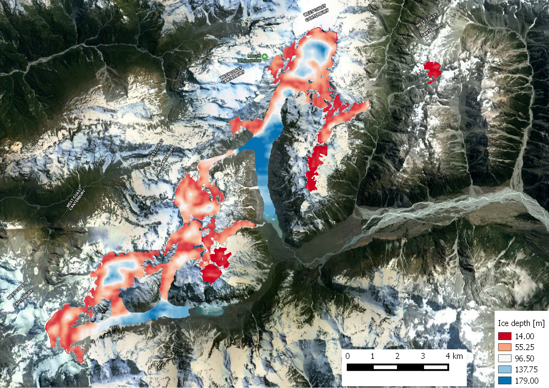
Figure 2 Example of glacier ice depth map as generated by GlabTop2-py.

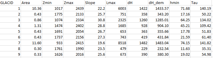
Figure 3 Example of glacier properties per GLACID in a csv-file as generated by GlabTop2-py.